EOPatch visualization

This tutorial showcases EOPatch visualization functionalities. We are going to load and visualize features from TestEOPatch.

%matplotlib inline

import os

from eolearn.core import EOPatch, FeatureType

EOPATCH_PATH = os.path.join("..", "..", "example_data", "TestEOPatch")

eopatch = EOPatch.load(EOPATCH_PATH)
eopatch

EOPatch(
  data={
    BANDS-S2-L1C: numpy.ndarray(shape=(68, 101, 100, 13), dtype=float32)
    CLP: numpy.ndarray(shape=(68, 101, 100, 1), dtype=float32)
    CLP_MULTI: numpy.ndarray(shape=(68, 101, 100, 1), dtype=float32)
    CLP_S2C: numpy.ndarray(shape=(68, 101, 100, 1), dtype=float32)
    NDVI: numpy.ndarray(shape=(68, 101, 100, 1), dtype=float32)
    REFERENCE_SCENES: numpy.ndarray(shape=(5, 101, 100, 13), dtype=float32)
  }
  mask={
    CLM: numpy.ndarray(shape=(68, 101, 100, 1), dtype=uint8)
    CLM_INTERSSIM: numpy.ndarray(shape=(68, 101, 100, 1), dtype=bool)
    CLM_MULTI: numpy.ndarray(shape=(68, 101, 100, 1), dtype=bool)
    CLM_S2C: numpy.ndarray(shape=(68, 101, 100, 1), dtype=bool)
    IS_DATA: numpy.ndarray(shape=(68, 101, 100, 1), dtype=uint8)
    IS_VALID: numpy.ndarray(shape=(68, 101, 100, 1), dtype=bool)
  }
  scalar={
    CLOUD_COVERAGE: numpy.ndarray(shape=(68, 1), dtype=float16)
  }
  label={
    IS_CLOUDLESS: numpy.ndarray(shape=(68, 1), dtype=bool)
    RANDOM_DIGIT: numpy.ndarray(shape=(68, 2), dtype=int8)
  }
  vector={
    CLM_VECTOR: geopandas.GeoDataFrame(columns=['TIMESTAMP', 'VALUE', 'geometry'], length=55, crs=EPSG:32633)
  }
  data_timeless={
    DEM: numpy.ndarray(shape=(101, 100, 1), dtype=float32)
    MAX_NDVI: numpy.ndarray(shape=(101, 100, 1), dtype=float64)
  }
  mask_timeless={
    LULC: numpy.ndarray(shape=(101, 100, 1), dtype=uint16)
    RANDOM_UINT8: numpy.ndarray(shape=(101, 100, 13), dtype=uint8)
    VALID_COUNT: numpy.ndarray(shape=(101, 100, 1), dtype=int64)
  }
  scalar_timeless={
    LULC_PERCENTAGE: numpy.ndarray(shape=(6,), dtype=float64)
  }
  label_timeless={
    LULC_COUNTS: numpy.ndarray(shape=(6,), dtype=int32)
  }
  vector_timeless={
    LULC: geopandas.GeoDataFrame(columns=['index', 'RABA_ID', 'AREA', 'DATE', 'LULC_ID', 'LULC_NAME', 'geometry'], length=88, crs=EPSG:32633)
  }
  meta_info={
    maxcc: 0.8
    service_type: 'wcs'
    size_x: '10m'
    size_y: '10m'
  }
  bbox=BBox(((465181.0522318204, 5079244.8912012065), (466180.53145382757, 5080254.63349641)), crs=CRS('32633'))
  timestamps=[datetime.datetime(2015, 7, 11, 10, 0, 8), ..., datetime.datetime(2017, 12, 22, 10, 4, 15)], length=68
)

Basics

All visualizations can be done simply by calling EOPatch.plot method, however calling this method still requires that Dependencies eo-learn[VISUALIZATION] are installed.

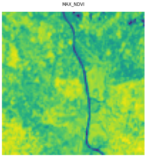
Plotting a simple timeless single-channel feature produces a single-image plot. Plotting method always returns a 2D grid of AxesSubplot objects which can be further customized before a plot is produced.

axes_grid = eopatch.plot((FeatureType.DATA_TIMELESS, "MAX_NDVI"))

print("A 2D grid:", axes_grid)

figure = axes_grid[0][0].figure
figure.set_dpi(40)

A 2D grid: [[<AxesSubplot:>]]

Plotting filters and configurations

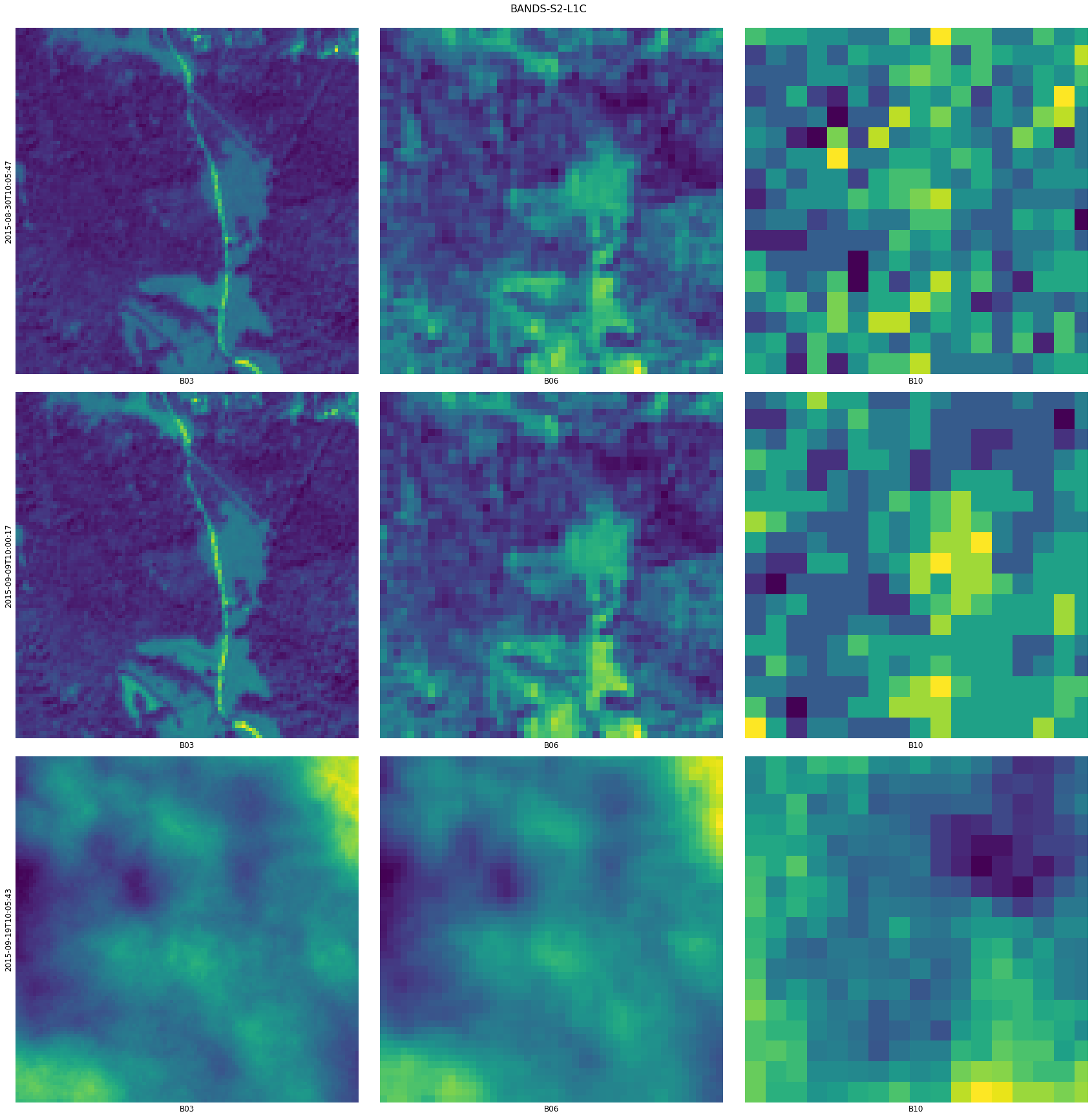
Let’s plot a feature containing Sentinel-2 bands. It will create a grid of subplots where every row contains images for the same timestamp and every column contains images from the same channel.

Because plotting a grid of 68 x 13 images would take too much time and memory we’ll use filters to plot only some timestamps and channels. Filtering parameters support either a slice object or a list of indices to keep. Additionally, we can write the names of channels to be written next to each image.

eopatch.plot(
    (FeatureType.DATA, "BANDS-S2-L1C"), times=slice(3, 6), channels=[2, 5, 10], channel_names=["B03", "B06", "B10"]
);

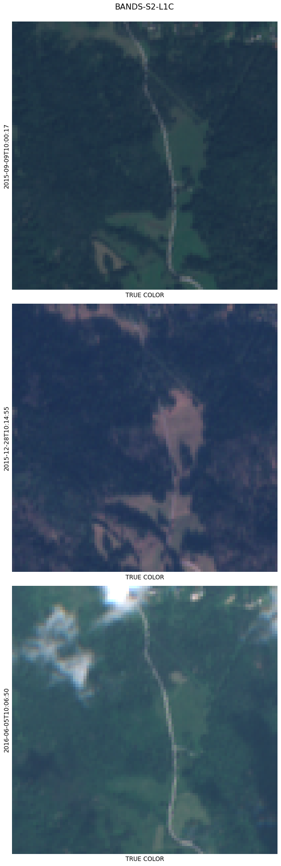
We can also select any 3 channels and plot RGB images.

eopatch.plot((FeatureType.DATA, "BANDS-S2-L1C"), times=[4, 10, 20], rgb=[3, 2, 1], channel_names=["TRUE COLOR"]);

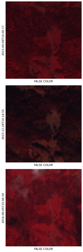
Plotting also supports plenty of advanced low-level configuration options. Those can be configured with a PlotConfig object.

from eolearn.visualization import PlotConfig

config = PlotConfig(subplot_width=5, subplot_height=5, rgb_factor=1, show_title=False)

eopatch.plot(
    (FeatureType.DATA, "BANDS-S2-L1C"), times=[4, 10, 20], rgb=[7, 3, 2], channel_names=["FALSE COLOR"], config=config
);

Types of plots

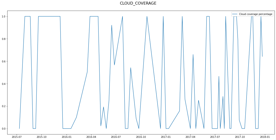
Next, let’s check what kind of plots other feature types produce. Non-spatial temporal raster features are plotted as time series of values.

eopatch.plot(
    (FeatureType.SCALAR, "CLOUD_COVERAGE"),
    channel_names=["Cloud coverage percentage"],
    config=PlotConfig(subplot_width=16),
);

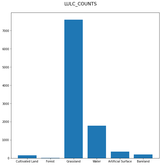
Timeless non-spatial raster features produce histogram plots.

eopatch.plot(
    (FeatureType.LABEL_TIMELESS, "LULC_COUNTS"),
    channel_names=["Cultivated Land", "Forest", "Grassland", "Water", "Artificial Surface", "Bareland"],
);

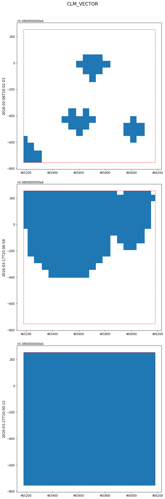
Vector features are plotted together with an EOPatch bounding box.

eopatch.plot((FeatureType.VECTOR, "CLM_VECTOR"), times=slice(6, 9));